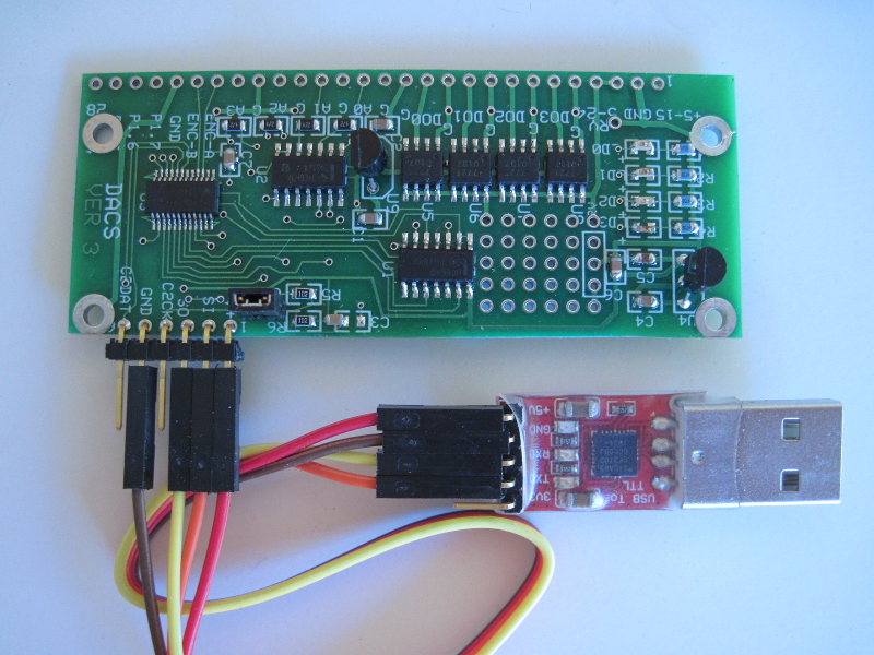
The Serial Data ACquisition System (DACS) module makes it easy to control devices and acquire data using a serial port and simple commands. The DACS module, shown above, has four digital outputs, six digital inputs and four analog inputs. The board also provides a temperature readout based on a sensor internal to the processor.
One use for the module is to manually monitor and control external circuitry using a serial terminal. The module can also perform automated monitoring and control using Linux shell scripts or PERL scripts.
For example, the serial port of a Raspberry Pi can periodically query the module for data and save it to a file. The data from the file is easily plotted with a program such as GNUplot. Plotted data, in the form of a JPEG image, can be displayed on a Web page to local or remote users. This manual describes how to use a bash shell script to acquire DACS data with a date/time stamp.
Page ii
(BLANK)
Page iii
Page iv
Page 1
The DACS Serial Data Acquisition and Control Board (DACS or DACS system) is a microprocessor-based system that provides an easy way to control outputs, monitor digital inputs and read analog voltages. The DACS board also provides a temperature reading based on the microprocessor's internal temperature sensor.
The DACS board uses a Silicon Laboratories C8051F850 processor to manage serial commands from the user and to control various inputs and outputs via connections to its 28 input and output (I/O) pins.
Digital outputs from the microprocessor are passed through a logic chip to ensure that outputs do not come up in the "on" state. Also, outputs are isolated from the board logic through high side FET switches that provide output drive for external circuitry such as relay boards or indicators. These switches allow output loads to share a common ground and protect against inductor switching transients, loss of power, load voltage reversal and overcurrent. The board includes LED indicators to provide on-board status display for each digital output. Outputs can be configured for normal or inverted logic.
Digital inputs are not conditioned, but are suitable for direct connection to three or five Volt logic outputs from external circuitry. Typically, inputs connect to field connections through an opto-isolator board.
Analog inputs are connected to the chip through an operatational amplifiers connected as voltage followers. These provide a high impedance input for user circuitry and also provide a low impedance drive for the chip's analog inputs. The analog input isolation also provides some protection for over-voltage input signals.
The temperature monitoring capability provides a reasonably accurate temperature reading based on the internal temperature sensor of the microprocessor (chip). More accurate readings depend upon performing a one-time single or dual point correction. This procedure is relatively straightforward and is described in this manual. A rough calibration is performed at the factory with a commercial thermocouple meter.
Once calibrated, the temperature sensor has been shown to agree well with commercial temperature monitoring instruments such as a thermocouple-based meter. Good agreement was also obtained with a laboratory-grade mercury thermometer. Calibrated accuracy is approximately one degree Celsius. Because chip power consumption is low (e.g., 20 milliwatts), innacuracy due to self-heating is considerably reduced.
Page 2
Assuming that you have just purchased a board, you may want to quickly check out some basic features and get a feel for how it works interactively.
First read the power and serial sections below to see how to connect power and a serial terminal to the board. In most cases, this is as simple as plugging in the supplied USB adapter to a USB port and bringing up a terminal that uses the resulting serial link. The terminal should be configured for operation at 19.2K baud with 8 data bits, no parity and 1 stop bit. You may also have to disable local character echoing.
With a terminal connected, entering a carriage return should produce a ">" prompt. Entering an "h" at this command prompt, followed by a space or carriage return, produces the main help screen. This screen provides a brief summary of the most frequently used commands. Also try entering "hx" to display the extended help screen. These two screens provide a basic overview of all of the commands that DACS can execute.
One useful command is the "t" command. It displays the current temperature in both Celsius and Fahrenheit. Note that there are no units attached to the numbers. This is because DACS is often used with scripts that produce log or plot files for which the units are of marginal use.
The outputs need to be connected to a separate supply and to output devices such as relays before they can be used. But, you can observe the action of the LEDs that show the state of the four outputs.
The easiest test of the LED indicators is to enter the "o+" command. This turns on all of the output drivers and their indicator LEDs. This command also illustrates the simple DACS command structure where the first character specifies the type of Input or Output (I/O) and the second character specifies an action ("+" for "turn on", in this case).
Now that you have turned on all of the indicators, use the "o-" command to turn them all back off again.
To display the state of the output drivers, enter the "o" command. Outputs that are turned on display a "1" and outputs that are off display a "0", with one symbol for each output. To specify one output, enter the I/O type, followed by the number of the output and the operation to perform. For example, enter "o2+" to turn on the driver and LED for output 2. Note that the four outputs are designated 0, 1, 2 and 3 (i.e., they are zero-indexed). Thus, the "o2+" command turns on the third LED.
Page 3
The "o2-" command turns off output 2 but there are three other ways to turn it off. Entering the "o2~" command toggles or reverses the sense of output two (i.e., on goes to off and off goes to on). Another way to turn off output 2 is to enter the "o-" command: that turns off all outputs. The "o~" command toggles all of the outputs. In this case, it will turn off output 2 but will also turn on output 0, 1 and 3.
We suggest experimenting with the "o" commands and observing their effect on the indicator LEDs. This is a good exercise before connecting relays or other devices to get an idea of the effect of the commands on the real outputs.
Now that you have a feel for how the commands operate, you can also experiment with others. At this point, you cannot do any harm but many of the commands do not provide any meaningful displays.
For example, you can enter the "v" command to display the voltages on the analog inputs. But, the voltages displayed will likely be a mix of meaningless values because the analog inputs are not connected to anything. Similarly, the "i" command shows the state of the digital inputs, but they all read "1" because the inputs are internally pulled up to the supply voltage. Nonetheless, experimenting with various commands can provide a basic feel for how DACS works.
Once you have a feel for how the commands work, you can connect an output to a relay to provide some immediate action.
To connect a relay, wire one side of the coil to an output and connect the other side to the ground for the "RV" supply. Ensure that the "RV" supply can furnish enough current to drive the relay (e.g., do not use the 5 Volts from the USB adapter).
Now try entering "o+" to activate all outputs. The relay should operate. To deactivate the relay, use the "o-" command or "o~" commands. Of course, you can also use the commands intended for controlling the specific relay you connected, For example use "o0-" or "o0~" for a relay connected to output 0.
Page 4
The DACS module features the following:
Assembled and Tested
The board is furnished assembled and tested with connections available on 0.1 inch-spaced holes on the board edges. This allows easy connection of wires, stake pins or 0.1 inch-spaced screw down connectors.
With stake pins soldered to the board edge, it can be inserted into a solderless breadboard or socket-mounted on a perforated carrier board. Photo 1 below shows the DACS board. Photo 2 below shows the DACS board socketed on a prototyping board with 0.1 inch screw down connectors mounted the I/O connections.
Serial Readout and Control
A serial port provides readout and control of digital and analog I/O, temperature, status and configuration. Serial commands are simple and can be issued manually via a terminal program or automatically via a command script (e.g., a Linux shell script). Responses have been designed for easy interpretation from a script or control processor. A help screen is available to list frequently-used commands, the current version and operational notes. An extended help screen covers less-used commands.
Versatile Display Formatting
Analog values can be displayed in counts or Volts. All analog voltages, digital inputs and output states can be displayed individually or on the same line as a group (e.g., all analogs on a single line). The state of any individual analog input, digital input or output can be displayed. A status command displays all I/O on a single line with each I/O group separated by a vertical bar delimiter. This allows easy logging and script processing.
Outputs
Outputs are controlled by four high-side FET switches. These are suitable for driving grounded loads of several amperes each and withstanding voltages up to 34 Volts. Outputs come up in an inactive state so that external circuitry is not accidentaly turned on when the DACS starts up or is rebooted. Outputs can be set to operate with reverse logic (i.e., a low output is "on"). Commands for controlling outputs allow setting, clearing or toggling individual outputs or all outputs simultaneously.
Page 5
Digital Inputs
There are six 5-Volt tolerant digital inputs. These inputs are unconditioned, with the assumption that the user's application will handle tasks such as opto-isolation for voltages higher than 3.3 or 5 Volts. Digital inputs may also require external noise filtering. Inputs are weakly pulled up internally for easy status reading of devices such as switches or relay contacts.
Analog Inputs
Four buffered analog inputs are available, each capable of being read to 13 bits. This typically provides millivolt resolution. Room temperature accuracy is on the order of 10 millivolts (or less) over the input range of 0 to 3 Volts. Accuracy is rated at better than one percent over typical temperature ranges and is compatible with scaling networks using one percent resistors.
Temperature
A temperature readout is available. The readout is based on the internal temperature sensor in the microprocessor chip. After performing a one-point calibration, we have found that temperature readings agree with thermocouple-based meters and a laboratory grade mercury thermometer to a degree Celsius. We rate the temperature accuracy at two degrees Celsius or less. Temperature readout is available in both degrees Celsius and Fahrenheit.
Documentation
The board features two on-line help screens. A main help screen documents the most frequently used commands and an extended help screen documents less used commands. This manual provides detailed descriptions of the board features, setup and command usage. The manual is formatted so that, when printed, it produces a correctly-paginated double-sided document. To see the formatted document, use the "print preview" option available on most browsers.
Page 6
The operation of the serial commands and the capabilities of each of the DACS inputs and outputs (I/O) is described more fully in the following sections. Because the descriptions in the following sections frequently refer to Schematic 1, we recommend downloading and printing a copy for reference.
Download the schematic by placing the mouse cursor on the link and performing a right-mouse-click/alternate-mouse-click on it. From the resulting menu, select the "Save Target As" or the "Save Link As" option. Once saved, you can print a copy for reference.
The schematic is not presented on a page in the manual as schematics are in many of our other manuals. This is because it does not scale down well to an A size format. However, two following pages are left blank so that a copy can be inserted in the manual if it is printed out.
Photo 3 shows the top side of the DACS circuit board. The silk screen notations help identify component placement, including the connector connections.
Page 7
Photo 1. Assembled DACS Board
Page 8
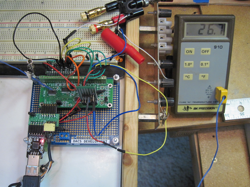
Photo 2. DACS Development System
Page 9
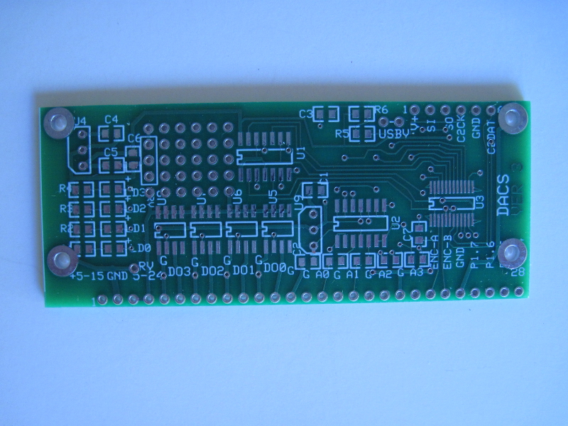
Photo 3. DACS Unassembled Circuit Board
Page 10
The Specifications for the DACS module are as follows:
Physical
The controller module measures approximately 1.25 by 3.125 inches (32 by 80 mm). As shown in Schematic 1, Power and I/O connections are available on a single-row 28-pin header located along the board's left edge. Serial and programming connections are available on a single row 6-pin header located along the board's right edge.
Power
Input power within the range of 5-15 Volts can be applied on the main I/O connector. With a jumper option set, 5 Volt power for the board is supplied from the serial/programming connector. Current consumption is approximately 7 milliamperes without indicator LEDs active. Indicator LEDs consume about 4 milliamperes each. Total consumption is under 25 milliamperes.
Power within the range of 5 to 34 Volts for output devices (such as relays) also connects to the main I/O connector.
Outputs
There are four outputs switched with high-side FET drivers. Output voltage range is 5 to 34 Volts. Output current up to 2.6 Amperes may be switched. Outputs are protected against over-temperature, inductive switching transients, reverse voltage and other common connection errors.
Digital Inputs
There are six logic-level digital inputs. Inputs are pulled up to 3.3 Volts internally but are 5-Volt tolerant.
Analog Inputs
There are four analog inputs. The input voltage range for analog inputs is 0 to 3 Volts. Resolution is 400 microvolts. Accuracy is typically less than one percent: inputs are suitable for use with 1% scaling resistors. Inputs are protected against brief overvoltages.
Temperature
A temperature reading is available that is derived from an on-chip temperature sensor. When calibrated according to instructions in this manual, temperature readings are typically better than 2 degrees Celsius.
Page 11
Page 12
Page 13
The following are the basic DACS design objectives:
Easy Operation and Hookup
The board can be easily connected for operation as a data acquisition system, requiring only board power, output load power and a serial connection. Thus, the user can easily read and control the DACS I/O as soon as it is hooked up.
Simple Operating Commands
The DACS commands typically consist of on or two characters. The characters for major functions are few and designed to be easy to remember and fast to enter from a terminal or from a control processor. A main help display describes the most-used DACS commands. An extended help screen describes less-used commands. The two help screens describe the entire command set.
High Functionality
Although major commands are simple, a full complement of commands provides monitoring and control of all functions, including option setting and retention in non-volatile memory. Thus, DACS can be customized for applications that require unique configurations while retaining operational simplicity for commonly-used functions.
Page 14
As shown in Schematic 1, all analog and digital I/O is available on the 28-pin connector, PL1, that consumes the entire left side of the board. Serial I/O and programmer connections are availble on PL2, the 6-pin BOBI interface connector near the bottom right side of the board.
To set up for operation, first connect 5 to 15 Volt power between the "VDD" pin of the PL1 I/O connector and PL1/2 (or any the ground pins on the same connector). Multiple grounds are not required.
As mentioned above, 5-Volt power can be furnished via the USB to serial connector. In this case, do not connect power to PL1 pin 1 (PL1/1). But, this pin can be used to feed 5 Volt power to other circuitry.
![]()
Because outputs typically operate at higher voltages and currents, they have their own separate power supply, labeled "RV" (relay voltage). Apply power for the outputs between the "RV" terminals, PL1/3 and 4, and a nearby ground (i.e., PL1/2 and/or PL5). Other PL1 grounds (e.g., analog grounds) are not recommended for the "RV" voltage connection.
Page 15
The DACS module requires a serial data link attached to a serial terminal program. The following describes how to connect the serial link hardware and configure a terminal program to operate with it.
As shown in Schematic 1, serial and C2 programmer connections are availble on PL2, the 6-pin BOBI interface connector near the bottom right side of the board. Serial connections are made to the SI (serial input), SO (serial output) and ground (GND) pins.
A USB to serial adapter based on the Silicon Laboratories CP210x chip set is furnished with each module. This can be used with a Windows or Linux PC to establish a serial link. A serial terminal connection using this adapter requires connecting this adapter to a USB port on the PC and configuring a terminal program to operate with it.
A direct serial connection, such as that available on the Raspberry Pi, can also be used with a terminal program to provide a terminal connection.
The following sections describe how to establish a serial data link using a USB to serial adapter or a direct hardware connection.
Each module is tested with the USB to serial adapter that we furnish. The serial connections between the adapter and the DACS module are left in place when the hardware is shipped. Thus, the wire connections from the serial adapter and the BOBI interface needn't concern you. But, you may want to note the connection color coding in the event that they are later disconnected.
You can also reconnect the wires without reference to the original connections by observing the data sense arrows shown on Schematic 1 and noting the designations on the adapter.
Most serial I/O designations are "board centric" in that outputs are from the board and inputs are to the board. This is the convention we use. Thus, an adapter connection labeled "TXD" is most likely the transmit output from the adapter. If this is the case, it would connect to pin 2, "SI" (serial input) to the BOBI connector.
If your connections do not work, you can try reversing the connections. Although we are obligated to warn that this has the potential to damage the hardware, we have done this on several adapters (and the direct connection to the Raspberry Pi) without damage.
Once the USB connection is established, Windows systems using the furnished adapter generally require installation of the "VCP" serial driver available at the Silicon Laboratories web site.
Page 16
Silicon Laboratories provides several application notes that discuss the operation and installation of CP210x drivers on Windows systems. The most applicable is AN335, titled "USB Driver Installation Methods." This discusses installation on various types of Windows systems, including XP. Detailed explanation of how to install drivers on Windows systems is beyond the scope of this manual.
Linux systems are somewhat easier. The USB-based serial connection is usually automatically configured when the adapter is plugged in. But, to configure the terminal program it is necessary to determine the device mapping.
Serial device mappings vary between Linux distributions but our PC running Debian maps the first com device as: /dev/ttyUSB0. Unless you have other USB to serial adapters attached, this is the most likely mapping for the adapter.
To find what serial devices you system has mapped, use something like: dmesg | grep "ttyUSB" or dmesg | grep "tty" at a command prompt.
The following section describes direct serial connections, including connection to a Raspberry Pi. Note that a USB connection can also be used with the Raspberry Pi and Beaglebone Black.
The serial data link can be implemented with a direct connection to a hardwired TTL-level serial port such as that available on the Raspberry Pi.
A direct serial connection to a hardwired port that operates at true RS-232 voltage levels requires a TTL to RS-232 adapter. These are inexpensive and commonly-available. They are discussed and shown in the manual for the BOBZ DCON product.
For direct TTL-level serial connections or connections to the TTL levels provided by an RS-232 adapter, connect the TTL data output to the "SI" pin and the TTL data input to the "SO" pin.
The Raspberry Pi serial connections are as follows:
If you are not sure of the Pi pin numbering, there are a number of pictorials on the internet that show it. The Pi has a single serial port which maps to "/dev/ttyAMA0." You can also use a USB to serial adapter for your Pi serial port.
Page 17
Once the serial link is established and the device or the "com" number is known, install a terminal program and configure it for the DACS serial settings.
Any terminal program such as Hyperterm, Procomm, PuTTY, or minicom (Linux) should work. We like PuTTY, which is available for both Windows and Linux. The minicom terminal program is a good choice for Linux systems because it is often already installed.
Configure the terminal program by setting the device (Linux) or "com" number (Windows). Configure the terminal program for 19200 baud with 8 data bits, no parity and one stop bit. Also disable local character echoing (DACS echos characters).
When configured and connected properly, entering a command elicits a response from the processor. For example, entering a carriage return (or space) gives a ">" prompt.
For users with Linux systems and minicom, we suggest starting it up as root in the configuration mode (i.e., "sudo minicom -s"). This allows you to set the device and baud rate and save it to the default configuration file.
With minicom, you can also save the current configuration as a named configuration file. These are named "minirc.xxx", where the "xxx" is a name you supply. Configuration files are normally stored in a location such as "/etc/minicom" and are specified as a command line parameter at startup.
For example, entering "minicom dac" at a shell prompt might be used to bring up minicom using a configuration file named "/etc/minirc.dac" specifying "/dev/ttyUSB0" as the serial port and configured for DACS operation.
There are many ways to to install a serial port and connect it to a terminal program for various hardware and software products. It is beyond the scope of this manual to describe all of the possible combinations. But, there are many detailed tutorials available on the Internet.
When power is first applied to DACS, it outputs the revision number and a "!" to signal a reboot. You can observe this startup message with the terminal program. Incorrect baud rates and other configuration errors, other than an incorrect device number, usually result in a display of "garbage" characters.
If the startup message appears to be correct, test the controller by entering the "h" (help) command. This displays a header containing the current version number, followed by a list of commonly-used commands. The version number is the date of the last firmware load and is displayed in YYMMDD format (e.g., 140525 for a firmware load date of May 25th, 2014).
Page 18
As shown in Schematic 1, all analog and digital I/O is available on the 28-pin connector, PL1.
Most connections are available on a 28-pin row along the left side of the board (PL1). A 6-pin row on the opposite board edge, PL2, provides connections for the serial port, 5 Volt power and the C2 programming interface. This 6-pin connection group is our standard "BOBI" interface.
A two-pin jumper, USBV, near PL2, allows the board to be powered from the BOBI interface. This power is typically derived from the same USB to serial adapter furnished with the DACS board. Connections to the USB to serial adapter are typically made with four socket-to-socket jumpers supplied with the adapter.
There are four small "mounting" holes near the board edges. These holes are not intended for mechanical mounting and do not presently fit any standard machine screw or standoff width: they are intended for soldering to stake pins when the board is mounted on a prototyping board. The large hole size provides some flexibility when soldering to the mounting pins.
The holes near the bottom of the board (nearest U3) connect to ground and can be used to carry ground between the DACS board and the prototyping board through a soldered pin connection(s). Although a small standoff can be fitted on these holes, do not rely on a standoff to carry ground to a prototyping board. Normally, ground connections to the prototyping board should be connected via the ground pins on PL1.
The board can be mounted on a prototyping board by soldering stake pins on PL1 and a row of socket headers on the prototyping board. With a row of stake pins soldered to PL1, the board can also be used with a solderless breadboard.
As shown in Photo 2, 0.1 inch-spaced screw-down connectors (not furnished) can be installed directly on the PL2 holes. This is the configuration used during development.
Page 19
Commands are designed to be easy to use and remember. A simple command structure also facilitates automated processing from a control computer such as a Raspberry Pi, Beaglebone or Arduino.
Entering "h" at any command prompt provides a list of the most-used DACS commands. Other less-used commands, such as those used for temperature calibration, are displayed with the "hx" (extended help) command.
A single character is used to monitor the state of all I/O of a particular type. For example, the "v" command displays the voltage on all of the analog inputs and the "o" command displays the state of all four digital outputs.
Individual I/O channels can also be queried and displayed. Commands to query individual inputs or outputs consists of two characters. The first character specifies the type of I/O (e.g., "o" for output) and the second character specifies the number (e.g., "3" for input or output 3). For example, the "v2" command displays the voltage on analog input 2 and the "o1" command displays the state of output 1.
Several three-character commands are available to control outputs. The first two characters of these commands specify the type and number, as above, and the last character specifies an operation. An operation of "+" turns an output on and a "-" turns an output off. An operation of "~" complements (reverses) an output.
Thus, the command "o3+" turns on output 3 and "o3-" or "o3~" turns it off again.
Commands can also act on all I/O of the same type. For example, the "o+" command turns on all outputs, the "o-" command turns them all off and the "o~" command complements all of them.
Responses do not have units attached to them. This is because one common use is to generate commands and read responses from to a control processor or a script (e.g., one running on a Linux platform such as a Raspberry Pi). The units are generally obvious and eliminating them often simplifies response processing. For example, responses captured by a script are often directly routed to a log file or a plot file with little or no additional processing.
Page 20
Commands execute as soon as a carriage return or a space is entered. Commands do not have embedded spaces. Because commands can execute with a space, multiple commands cannot be executed on the same line. Either a space or a carriage return can be used to terminate a command issued from a control processor or script.
For valid commands, the DACS command interpreter responds with the requested information followed by a space and the command termination sequence. The termination sequence is a carriage return, a line feed and a ">" character.
For unrecognized commands, the response is a "?" followed by the termination sequence. For a reboot, the response is a "!" followed by the termination sequence. There are no hidden commands: commands used for factory calibration and test are embedded in the firmware but disabled before units are shipped.
The character "n" is reserved and does not appear as part of any command. This convention is used because "n" is used on the help screen (and in this manual) to designate input or output numbers used within a command. When used in this way in the manual, the "n" is italicized to emphasize that it is a placeholder for a number.
For example, the command for turning an output on appears as "on+", where "n" is the channel number (0 to 3). Thus, the command "o2+" turns on output 2.
As noted above, commands normally consist of one, two or three characters. Single character commands display all I/O of a particular type. For example, the "a" command provides the input counts for all four analog channels.
Two character commands may have different contexts, depending on the I/O type. For example, the "o~" command toggles all of the digital outputs and the "tc" commands requests display of the chip temperature in Celsius. Typically, the second character is the number of the I/O channel or a type qualifier for the first character. For example, "i5" specifies the display of input 5 and "tg" displays averaged temperatures.
Three character commands are rare. There are only four of them and three are associated with controlling outputs. For output control, the third character denotes the operation to be performed (e.g., "+" for turning an output on). For example, the command "o2+" turns on output 2.
The "dat" command is a special three-character command that shows option and calibration data. Commands exceeding three characters are reserved for configuration options such as "normal" and "inverted" to set the sense of the output logic.
Page 21
As noted above, the response to an unrecognized command is a "?" followed by the termination sequence. For automated applications where the commands and responses are issued and processed by a control processor or script, the "?" character represents a command error to the contnroller.
The control processor or script may also need to detect startup, reset, power cycling or version date.
At startup, the processor displays "DACS", followed by the revision date, coded as a YYMMDD, where 140525 (for example) would represent May 25th, 2014. The control processor or script can use the version date for applications that are version sensitive.
Following the version, DACS outputs a "!" character to allow a control processor to detect a restart due to power cycling or in response to a reboot command. The "!" character is followed by the termination sequence.
Thus, responses are detected by capturing the last four characters of a response and examining the first character captured. The last three characters are always the termination sequence and do not change.
For a normal response, the first character is a space, for a command error the first character is a "?" and for a reboot the first character is a "!" (this is not necessarily an error). The last character of a response should always be a ">" character.
Note that the "r" command resets the processor. Issuing an "r" command and checking for a "!" response string can be used to verify that the serial link and processor connection are active. This is often done if there is no response to a command. A less obtrusive way to check the link is to issue a carriage return or a space: the response for a working link is the termination sequence.
Page 22
There are six digital inputs, designated as "i0" through "i5", and they can be monitored either as a group or as individual inputs.
The "i" command shows the state of all inputs as a series of "1" or "0" characters. These read left to right as I0, I1, I2, I3, I4 and I5.
The "in" command displays the state of individual inputs, where "n" designates the input number from 0 to 5. For example, "i4" displays the state of input 4.
Page 23
Schematic 1 shows the input connections.
The six digital inputs are designated on the schematic as I0 to I5 and connect on PL1 from pins 22 to 28. Pin 24 is the common ground point for inputs.
Inputs are internally pulled up to 3.3 Volts by enabling the processor's "weak pullup" option. Without any connections to the digital inputs, all inputs should read "1" when displayed with the "i" or "in" commands.
For example, entering "i3" reads the state of input 3. If a "1" is returned, this indicates that input 3 is high; if a "0" is returned, input 3 has been forced low (i.e., grounded). Inputs reading "1" may be pulled high by a device driving the inputs. However, a reading of "1" may also indicate an unconnected input.
Observe that shorting pin 27 (I4) to pin 24 (ground) causes I4 to read "0" when queried with the "i4" or "i" commands.
Inputs are 5-Volt tolerant. If the inputs must be pulled up harder than the weak pullups provide, they can be connected through a resistor to a 5-Volt or 3.3-Volt supply. If used, a "hard" pullup resistor of 10K is sufficient for most applications.
The 3.3 Volts from the board regulator is not available on PL1. This prevents inadvertent overload of the internal digital regulator. If the inputs are pulled up externally to 3.3 Volts, we recommend using a separate 78L3.3 regulator. Many USB to serial adapters also provide regulated 3.3 Volts that can be used for pullups.
Applying more than 5 Volts to any input may damage the processor. To prevent this, isolate inputs with added circuitry such as opto-isolators or logic gates. Opto isolation is ideal for connections susceptible voltage spikes or external noise.
To reduce radio frequency interference, bypass susceptible inputs to ground through a 0.01 to 0.1 microfarad capacitor. Install the bypass as near as possible to the PL1 connections.
Avoid applying negative voltages, no matter how small, to inputs. The potential for input damage due to negative inputs can be minimized by connecting a reverse-biased diode from a susceptible input to ground.
Often, a pair of reverse-biased diodes are used to limit both positive and negative excursions on an input. Small dual-diode packages such as the MMBD4148SE can be used for this type of protection. Other types of protection or opto-isolation may be required, depending on the application.
Page 24
Inputs are often used to verify the operation of devices controlled by the outputs. For example, an input may be used to monitor the voltage applied to a solenoid or the output from a digital soil moisture probe.
Another typical use for digital inputs is to monitor the position of a switch or the state of an isolated contact on a relay. For example, if a pilot relay is used to turn on a load, the application of power to the relay can be monitored using an auxiliary contact.
This type of monitoring is simple to do but generally less effective than directly monitoring the controlled device or desired result (e.g, the rotation of a motor shaft or the resistance of a moisture probe). Most of these "long loop" applications require a digital input to be derived with additional circuitry.
Schematic 2 shows a simple way to locally monitor a DACS output. For local monitoring, the output and input can have a common ground reference. For the input connection shown, connect the isolated transistor's emitter to the local board ground and connect the transistor's collector directly to an input. Because the inputs are internally pulled up, there is no need for a separate resistor from the collector to 3.3 Volts.
Note the extra resistor from the transistor's base to ground: it is needed to prevent leakage current from pulling the input low. This can happen because the weak pullups are easily pulled toward ground by even a small collector current.
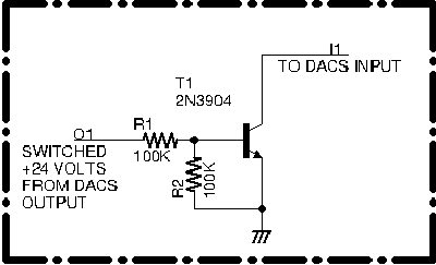
Schematic 2. Monitoring an Output with an Input
Page 25
Opto isolation is a good way to monitor voltages that may be too high or too noisy for direct connection to inputs. Opto-isolation is effective is when monitoring a voltage at some distance from the board. This breaks ground loops and minimizes noise pickup and transients induced in long wiring runs.
One common application is to monitor the state of an output operating at a higher voltage than the inputs can tolerate or monitoring a voltage that is remote from the board.
For example, an output operating 24 Volt relay may need to be monitored remotely at the relay. To do this, connect the positive side of the remote relay to the anode of the isolator's internal LED through an appropriate limiting resistor. Connect the cathode lead of the isolator's LED to the ground side of the remote relay. This activates the isolator when the remote output is energized.
Schematic 5 Shows the basic connection for local monitoring of an output with an opto-isolator. The connection shown can be used when it is possible to operate with a common ground reference between the input and output.
For remote monitoring, the ground for the LED cathode and the ground for the transistor's emitter should be tied to separate ground points.
The connection in Schematic 5 can be used when it is more convenient to use an opto-isolated connection instead of the circuit given in Schematic 2. Like the circuit in Schematic 2, the input circuit using the isolator provides voltage level conversion.
The on-board breadboarding area is a good place to mount the transistor or opto-isolator and their associated resistors. Photo 2 shows a small PCB mounted in the breadboarding area that mounts the components shown in Schematic 2.
Application Note 3 describes how to bring out DACS I/O connections to screw-down terminals. This allows all DACS I/O to be conveniently brought out in a compact format.
On the board silk screen, inputs "I0" and "I1" may be labeled "ENC-A" and "ENC-B", respectively (Versions 2 and 3). This designates connection points for an incremental encoder extension that is not implemented. For reference, use the "I0" and "I1" designations on Schematic 1.
Page 26
There are four outputs that connect to pins on the I/O connector. Outputs are powered by a separate power supply that terminates on pins 3 and 4 of the I/O connector. The output drivers allow loads to be connected with a common ground. The outputs are also easy to use because they are protected against most common connection errors and operational challenges such as inductive load spikes.
Outputs are controlled and monitored with commands that begin with an "o" prefix. The four digital outputs, designated "o0" through "o3", can be monitored and controlled individually or as a group.
In the following, an "n" character embedded in a command designates the output number. For example, "on" designates the commands "o0", "o1", "o2" and "o3", where the numbers 0 to 3 are substituted for the "n" in the command.
Page 27
To display the state of all outputs, enter the "o" command. The outputs are displayed in "o0 o1 o2 o3" order. A "1" indicates outputs with voltage applied to them and a "0" indicates deactivated outputs. Note that the on-board LED indicators are derived from the state of the microprocessor's output pins and not directly from the load outputs. For a direct monitoring circuit, see the Input section.
To display the state of a single output, enter the "on" command, where "n" specifies the output number from 0 to 3. For example, the "o3" command displays output 3.
On-board LEDs indicate the output states. Except for operation in the inverted mode, outputs that are active are indicated by an illuminated LED. Indication in the inverted mode is discussed below.
One problem with using a microprocessor to control outputs is the indeterminate output state of the microprocessor outputs at startup. This can result in momentary glitches in the outputs during a processor reset. To mitigate this, the microprocessor outputs are fed through an exclusive-or logic chip before they are fed to the output drivers.
As shown in Schematic 1, the exclusive-or chip, U1, has one side of each of its four gates fed to a microprocessor output. Thus, as the chip reboots, U1 will not activate its outputs as chip output voltages change.
The LED indicators are driven from the output of U1 so that they directly display the output used to drive the 772 chips.
Page 28
The characters "+" and "-" are used to designate on/off actions. The "~" character designates an output to be complemented ("on" goes to "off", "off" goes to "on").
The "o+" command activates all outputs; the "o-" command deactivates all outputs. The "o~" command toggles (complements or reverses) all outputs. Note that, for most control applications, the "o~" command is of limited usefulness.
To activate an output, use the "on+" command, where "n" designates the output to activate, from 0 to 3. For example, the "o0+" command activates output 0. Similarly, the "o3+" command activates output 3.
To deactivate an individual output, use the "on-" command, where "n" designates the output to deactivate. For example, "o1-" deactivates output 1.
Note: output commands cannot be mixed on a line because command input terminates on entry of a space or a carriage return.
To toggle (complement) an output enter the "on~" command, where "n" designates the output to complement. For example, the "o2~" command toggles output 2.
Page 29
Outputs are controlled by BSP772T high-side FET switches. Because loads are protected against inductive transients, outputs can directly connect to relay coils and most other inductive loads. The 772 drives an N-channel output FET from a logic-level input and provides various protection measures such as reverse voltage protection.
The outputs are rated for a supply voltage up to 36 Volts (40 Volts maximum) and a supply current of 2.6 Amperes. We test outputs with 24 Volt relays.
The output drive circuitry has its own gate voltage drive, reducing the on state resistance of the output FET to approximately 60 milliohms. For most applications, the drop across the output switching device can be ignored.
Because the output voltage and currents are typically different from that used by the DACS module, the output voltage supply connects on two separate I/O pins.
As shown in Schematic 1, the output supply connection pins are PL1/3 and PL1/4. These pins are designated "RV" (relay voltage) on the schematic and board. Pin PL1/5 is the ground connection for the "RV" supply. Use of other ground pins is not recommended.
Because the outputs switch their loads to the high-side of the supply, one side of each load can be connected to ground. Thus, with 24 Volts DC applied between pin "RV" and ground, each output can directly drive a 24 Volt relay connected to ground.
Here are some of the features of the ouput drivers:
Page 30
Output loads, such as relay coils, can directly connect to the PL1 I/O connector pins designated for outputs, D0 (PL1/12), D1 (PL1/10), D2 (PL1/8) and D3 (PL1/6). Note that the D0 to D3 connections appear in reverse connection order on PL1. Ground connections are available adjacent to each output connection.
It is a common practice to monitor the state of outputs with off-board LEDs. This is desirable for a number of reasons. The most important reason is to provide direct indication of a voltage applied to an output. The on-board indicator LEDs indicate only what the output is supposed to be and may not indicate correctly if, for example, the relay voltage is inoperative or not connected to the board.
To indicate an output voltage with an external LED, connect the output to the anode of the LED through a limiting resistor and connect the LED cathode to ground.The size of the limiting resistor is determined by the output voltage, type of LED and desired brightness.
For example, using a supply voltage of 24 Volts, a red LED and a current of approximately 10 milliamperes, the LED limiting resistor would be approximately 2.2K Ohms. See the Inputs section for monitoring outputs with DACS inputs.
Schematic 3 shows how to connect an outboard indicator LED to an output.
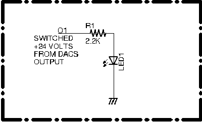
Schematic 3. LED Output Indicator
Page 31
Schematic 4 shows how to use an opto isolator to provide an inverted logic output. This circuit provides a suitable output for devices requiring inverted logic but it does not provide isolation.
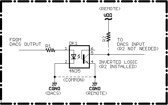
Schematic 4. Opto Isolator I/O
Page 32
Schematic 5 shows the circuitry for a typical opto-isolated relay board. In this case, the isolated relays operate when the cathode end of an isolator LED is grounded.
Because DACS outputs float when they are off, it is awkward to use them to directly drive the relay boards inputs. A better way to drive the inputs is to use an opto-isolator as shown in the schematic. Another way to drive the inputs is to use a transistor and two resistors, as shown in Schematic 2. The transistor driver is recommended only if the relay board and the DACS board are relatively close.
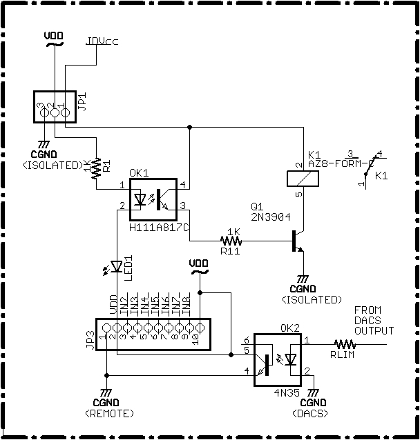
Schematic 5. Opto Isolator Relay Output
Page 33
Analog inputs are monitored with commands that begin with an "a" or "v" prefix. There are four analog inputs, designated either as "a0" through "a3" or as "v0" through "v3", depending on whether counts ("a" commands) or voltages ("v" commands) are requested.
As with previous commands, an "n" character embedded in a command indicates the output number. For example, "an" designates the commands "a0", "a1", "a2" and "a3", where the numbers 0 to 3 are substituted for the "n" after the analog count prefix.
The analog inputs are connected on connector PL1 on pins 15 (A0), 17 (A1), 19 (A2) and 21 (A3). Pins 14, 16, 18 and 20 are grounds to facilitate analog input connections and help maintain a one-point grounding configuration.
Page 34
Inputs are conditioned by an OPA4317 operational amplifier configured as a unity gain follower. The amplifier is a rated for rail to rail operation and features very low (near zero) drift, low offset voltage (20 microvolts) and low quiescent current (35 microamperes).
Momentary input voltages greater than the supply voltage (3.3 Volts) can be tolerated on the inputs provided that the input current is limited to 10 milliamperes. Input protection resistors are wired in series with the inputs per the manufacturer's recommendation. These protection resistors are designated R7 to R10 on Schematic 1. The outputs of the follower amplifiers are fed to the 850 chip's analog input pins (P1.0 to P1.3).
The inputs use the 1.65 Volt internal reference and a gain of 0.5 to provide an analog input range of 0 to 3.3 Volts. Because the supply voltage may be less than 3.3 Volts, the analog inputs are specified for operation only in the range from 0 to 3.0 Volts. Depending on the voltage regulator's output, readings above this (e.g., 3.1 Volts) may be usable, but extended ranges must must be determined by the user on a case-by-case basis.
The analogs are set up for 13-bit readings (dithered 12-bit operation, as explained in the Silicon Laboratories manual). This provides a basic resolution of 3.3/8192 = 400 microvolts. Accuracy is a bit more difficult to predict because it depends on many variables such as chip manufacturing, temperature, converter offset and slope errors, etc.
We have performed measurements at room temperature for a small number of modules using an Electronic Development Corporation (EDC) Low Impedance DC Millivolt Standard and an Agilent 34410A 6 1/2 Digit Multimeter. Reading errors were within a few millivolts of the measured inputs. As expected, maximum error was at zero (zero offset) and was typically 2.8 to 3.2 millivolts (7 or 8 counts). The software compensates somewhat for this non-zero reading.
The observed maximum error corresponds to an accuracy of approximately (3 millivolts)/(3000 millivolts) = 0.1 percent. But, the actual accuracy can be expected to be less than this, depending on the factors given above.
The DACS module was designed to provide overall accuracy of less than a percent so that 1 percent resistors can be used for voltage scaling. If greater accuracy is required, modules should be individually characterized over the range of conditions expected during operation.
Page 35
Use the "v" command to display the voltages on all four analog inputs. The ordering is: v0 v1 v2 v3 .
Use the "vn" series of commands to display the voltage on an individual input, where "n" designates the desired input. For example, enter "v3" to display the voltage on input 3 and "v0" to display the voltage on input 0.
Note that the voltages do not have units associated with them. Voltages can be displayed as fractional millivolts but the last digits typically change in increments of approximately 400 microvolts (0.4 millivolt) on successive reads. This incremental change results from maximum resolution of the converter and a typical reading variation of a few counts. This can be observed in more detail with the "counts" commands in the following section.
Page 36
It is sometimes useful to observe the counts returned by the analog to digital converter. For example, when an analog value is requested from a control processor. There are several commands to return analog counts, depending on whether all inputs or individual inputs are to be examined.
Additional command variations provide averaged readings, raw (not averaged) readings and a series of consecutive readings. The analog counts facility is primarily used when a control processor requires a value but it is not convenient to convert a multi-digit decimal value to a count.
Refer to the extended help menu for a summary of commands for displaying analog counts.
Single value count readings, including average values, are displayed in hexadecimal. Multiple readings are displayed in both decimal and hexadecimal because these are likely to be examined by the user, not processed by a script or control processor. Hexadecimal readings are prefixed with a "$" character (this corresponds to a "0x" prefix for hex numbers in C and other computer languages).
Use the "a" command to display the counts for all four analog inputs. These counts are raw (e.g., the result of a single reading for each input).
Use the "an" series of commands to display the counts for an individual input, where "n" designates the desired input. For example, enter "a3" to display the counts for input 3 and "a0" to display the counts for input 0.
Use the "arn" series of commands to display 32 consecutive readings for a specified analog input, where the "n" in the command designates the input from 0 to 3. Executing this command for an input reveals reading-to-reading variations and can be used to examine how input averaging influences displayed results. Another use for displaying consecutive readings is to detect high noise levels on individual inputs.
Typically, when inputs are driven from a stable low-impedance source, readings vary between 0 and 5 counts, corresponding to reading variations of 0 to 2 millivolts.
It is sometimes useful to see heavily averaged readings. Use the "ag" command to display the averaged counts for all four analog inputs. Each reading corresponds to 32 readings and is rounded to the nearest count. Readings are in hexadecimal for convenient reading and conversion from a control processor or script.
Use the "agn" series of commands to see averaged counts for an individual channel, where "n" designates the desired input from 0 to 3. For example the "ag2" command displays the averaged counts on analog input 2.
Page 37
Each DACS unit is calibrated for a full-scale reading of 3.000 Volts with a precision 3-Volt source. To achieve proper scaling for variations in the on-board voltage reference, the analog scaling factor, in millivolts/count, is adjusted and saved in memory. We refer to this scaling factor as "ascale" (analog scale). It can be viewed with the "dat" command: it is the field starting with an "a".
For example, entering "dat" might display a hexadecimal number such as "$9dd8." Converting the hexadecimal scaling factor to decimal (40,408) reveals the analog scaling factor, 0.00040408 Volts/count, scaled up by 10 to the 9th power. This is the scaling value used to calculate voltages from analog counts.
The analog scaling constant is set at the factory and cannot be changed by the user. Its value is of significance only when performing a one-point temperature calibration or when a control processor must convert analog counts to a voltage.
Page 38
The software is capable of displaying the voltage for a given number of counts to the highest resolution of the converter. This is approximately 400 microvolts. Variations of a few counts are common, especially if there is any noise on the input. Most applications do not need to read out the voltage to a high resolution and a resolution of millivolts is adequate.
The default resolution setting displays three digits after the decimal point with the last digit representing millivolts. In some cases, especially during tests at our labs, higher resolution is desirable. In this case, it is possible to get higher resolution by entering the "high" command. This provides a readout of five digits after the decimal point.
Use the "low" command to reset to low resolution.
To display the current resolution setting use the "dat" command. The resolution field starts with a "r" character and displays either "high" or "low", depending on the current setting.
You can also restore the default setting of "low" using the "%" (restore defaults) command. To save the current resolution setting, use the "!" command.
Note that just because a voltage is displayed to a high number of digits, this does not mean that the reading is accurate to that number of digits. The typical accuracy of a calibrated unit operating at room temperature is on the order of 10 millivolts. Thus, the low resolution display is more representative of the actual voltage.
Page 39
Use the "t" command to display the temperature in both degrees Celsius and Fahrenheit. Because of the 13-bit resolution used for a single temperature reading, single readings may vary. To smooth out these variations the displayed result is the average of multiple temperature readings.
Use the "tc" command to display the temperature in degrees Celsius. Because of the 13-bit resolution used for a single temperature reading, single readings may vary. To smooth out these variations the displayed result is the average of multiple temperature readings.
Enter "tf" to display the temperature in degrees Fahrenheit. As with the Celsius display, the Fahrenheit temperature is an average of multiple temperature readings.
Enter "tg" to display the averaged temperature count for 32 consecutive readings in hexadecimal.
Enter "tr" to display 32 consecutive temperature count measurements in both decimal and hexadecimal.
Enter "ts" to display the raw temperature count, in hexadecimal, for a single temperature reading.
Use the "tz" command to set the offset for the zero degree Celsius, as described below. The offset value is entered as a four-digit hexadecimal number immediately after "tz" is executed. The value entry automatically terminates and displays the current temperature.
Page 40
To improve temperature reading accuracy, it may be necessary to perform a one-point temperature calibration. Performing this calibration can improve temperature accuracy, often providing readings that are accurate to one degree Celsius.
Temperature calibration is described in more detail in the Silicon Laboratories Application Note titled "Accuracy Considerations for Microcontroller-Based Temperature Sensors." This note also describes how to interface to other temperature sensors, including those that provide a direct voltage output that can be measured with an analog input.
The purpose of a one-point calibration is to determine and compensate for the offset count at zero degrees Celsius. The change in analog voltage for each degree change is very stable, but it does not start at zero for a temperature of zero degrees Celsius. Because of this, the zero crossing value must be subtracted from the analog temperature count before applying the slope constant to calculate temperature.
The datasheet specifies a typical temperature sensor slope of 2.85 millivolts per degree Celsius. This constant is incorporated into the temperature display algorithm. Because the variation of this constant is slight (i.e., 70 microvolts), the 2.85 mV/degC slope value is used without correction in temperature calculations.
Of more significance in temperature calculation is the variation in the internal voltage reference used to calculate analog voltages. The nominal value of the voltage reference is 1.65 Volts but the datasheet gives a minimum/maximum range of 1.62 to 1.68 Volts. Slight variations of this reference can affect temperature calculations.
These variations are of minimal concern to the user because each unit is calibrated with a precision voltage reference to produce an accurate conversion of analog counts to Volts using the processor's internal reference. Calibration calculations in the following sections assume that the analog conversion constant unique to each module is used. A scaled version of the "millivolts/count" constant can be viewed with the "dat" command, as described above.
An accurate zero degree offset can be calculated using: 1. The analog scaling constant, 2. A single accurate temperature measurement and 3. A counts reading. The calculated offset can be used to change the offset used in the temperature conversion routine. After changing the offset, it can be saved to configuration memory so that future temperature displays are more accurate.
Note: A one-point calibration may not be necessary. A one-point temperature calibration is performed for each unit after the analog scaling factor has been determined. The resulting temperature is compared with a BK Precision Model 910 Temperature Meter. This meter uses a thermocouple: the thermocouple is placed on the chip during one-point measurement and during subsequent verification of the calculated offset.
Page 41
The most direct (but not necessarily the most convenient) way to determine the zero degree count is to immerse the board in an ice bath. During development we did this to compare the result with a one-point calculation at a known temperature.
You may also find this type of direct measurement instructive. To measure temperature in an ice bath, put the board in a lightweight watertight plastic bag with the bag's neck wrapped around the umbilical cable for power, ground and serial connections.
The wrap should be loose and can be easily held in place with a rubber band, tie wrap or electrical tape. If using the USB to serial adapter to connect to the DACS, the umbilical simply consists of the USB cable.
The loose wrapping allows air passage at the umbilical tie-off point to allow air to escape as it closely forms around the board under water pressure. The purpose of the bag is to provide secondary protection against condensation or water leakage in the immersion bag (described next).
Place the bagged board and its umbilical inside a second plastic bag, the "immersion bag." The umbilical cable routes out the neck of this bag. The immersion bag does not have to be tied to the umbilical wires: they route out of the top of the bag, which can be kept open. But, the top of the bag should extend some distance from the ice bath to avoid getting water inside.
Page 42
Place the immersion bag in the bath so that the icewater slurry presses against the immersion bag and the inner bag. This ensures good thermal contact. The bottom of the immersion bag can be weighted down to ensure that bath presses against the immersion bag. Take care that the neck of the immersion bag is kept well away from the bath to keep water from entering at the top.
Once the immersion bag has been in the bath for a while, measure the averaged temperature counts with the "tg" command. You can check for stability by using the "t" command at periodic intervals or by periodiclally entering the "tr" command to observe variations between readings. Use the reading obtained when consecutive readings show that the temperature has stabilized.
For our ice bath, we used an insulated cooler used for a six-pack of soda cans. When packed just over half full with an icewater slurry, we found that the board temperature stabilized in about 30 minutes. The thermal time constant of the bath itself exceeded one hour. Note that immersion in a temperature-stable water bath is also useful for performing a one-point calibration at a temperature other than freezing.
The "zero degree offset" temperature was approximately one or two tenths of a degree above freezing, as indicated by both a laboratory grade thermometer and a thermocouple-based meter. We reduced this reading by one count to compensate for the fact that the bath does not reach exactly zero degrees Celsius.
Use the "tz" command to set the temperature count for zero degrees Celsius.
This command allows entry of a hexadecimal constant corresponding to the zero degree offset. Enter "tz" followed by either a space or a carriage return. The command processor waits for entry of the four-digit hexadecimal zero count and then automatically terminates input. On input termination, the temperature is displayed for the zero degree offset just entered. This makes it easier to check the results and to identify entry errors.
For example, assuming that the new zero count is $06b8, enter: "tz 06b8". When the last digit is entered, data entry is automatically terminated and the resulting temperature is displayed, followed by the normal entry prompt.
You can directly verify the entry with the "dat" command. This displays the zero degree crossing point in the field labeled "z." If there is an entry error, re-enter or use the "%" command to restore the default zero crossing count.
After verifying the zero degree offset, save it to configuration memory with the "!" command. This ensures that, when the processor reboots, the corrected zero degree offset is used instead of the default. To verify this, enter the "r" command to reboot the processor and then use the "dat" command to display the zero offset.
Page 43
Determining the zero crossing point using an ice bath is instructive (and fun), but not necessary. The zero crossing offset can be determined using any accurate temperature measurement and a straightforward calculation.
A one-point calibration is performed by calculating the offset using a known accurate temperature, the reading for this temperature, and the analog scaling factor (read with the "dat" command). The one-point temperature calibration calculation is outlined below in Figure 1.
Once the zero degree offset count is known, use the "tz" command to enter the new value in hexadecimal. To enter the value, type "tz" followed by a space or a carriage return and then immediately type the four hex digits. After the last digit is entered, the entry is automatically terminated, displaying the temperature and the normal prompt.
Use the "dat" command to verify correct entry. Other than the automatic temperature readout, there is no other error checking. Do not be concerned about a data entry error: either re-enter the value, restore the default value or reset the processor (to restore the default or the last-saved zero count).
Assuming that the entry is correct, save it with the "!" command. Verify that it is correctly restored at startup by resetting the processor with the "r" command and then using "dat" to display the value (it is the data field identified with a "z" character).
The default zero crossing offset can be restored with the "%" command. Note that, if the default is restored and you want to use it permanently, you must save it with the "!" command.
Once a zero count is saved to flash configuration memory, it is restored at startup.
Page 44
  1. This calculation determines the count offset for a temperature of zero
     degrees Celsius, as outlined in the datasheet.

  2. From the datasheet:

      A. temperature (degC) = [Vtemp (mV) - Voffset (mV)]/[slope (mV/degC)]

      B. Solving for offset voltage: Voffset = Vtemp - (temperature)(slope)

      C. Converting voltages to counts using the A/D scaling constant,
         ascale, and the counts/degC (c/d):
            + c/d = [temperature slope (mV/degC)][ascale (counts/mV)]
            + offset counts = temp. counts - [temp. (degC)][c/d (counts/degC)]

  3.  Example:

      A. Assume the following:
            + The one-point temperature reading is 26.7 Degrees Celsius.
            + The "ts" command displays the raw temperature count as $0774
            + The scaling factor is $40408.  As shown in B, below, this corresponds
               to a reference of 3.31 Volts (2 x 1.6551 Volts),
               The agen scaling constant is determined at the factory and is
               displayed in the "a" data field with the "dat" command.

      B. Thus:
           + ascale = (3310.2 mV)/($2000 counts) = 0.404077 mV/count
           + c/d    = (2.85 mV/degC)/(0.404077 mV/count) =~ 7.0531 counts/degC

      C. zero degree offset count = $0774 - (26.7 DegC)(7.0530588 counts/degC)
                                  = $0774 - $bc = $06b8 (default)

      D. Note that the zero degree offset depends heavily on the analog scaling
         factor, ascale.
Figure 1. One Point Temperature Calibration
Page 45
Use the "h" command to display the most frequently used commands. Use the "hx" command to display commands that are used less frequently. These two screens cover all user commands.
To save current configuration options, enter the "!" command. With this command, the current configuration will be restored at startup. User configuration options include the following:
Use the "!" command to save the current configuration.
Note: Once any option is saved, it is restored from flash at startup.
Use the "%" command to restore factory default values (e.g., for normal configuration and default temperature calibration constant).
The configuration defaults are:
Use the "r" command to do a software reset of the processor. This command can be used in a script to verify module and serial link operability by detecting the "!" character at the end of the reboot response. For applications that may be version sensitive, the version can also be read from the startup message.
Note that, during a software reset, the supply voltage to the module does not change. For applications using inverted logic, however, outputs may briefly "glitch" if the supply to the switched outputs is not managed properly.
Page 46
Use the "s" (status) command to display all I/O on a single line. The I/O types are separated by a "|" character to make it easier for a script to process.
Use the "dat" command to display DACS configuration data. Configuration data consists of the following:
The items above are displayed in the order given. The data format is also given in the help screen. On the display, each item is contained within "|" delimiters to make it easier for a script to parse out individual fields. Each item is also associated with a "hint" character. For example, the serial number is prefixed with an "s" and the version is prefixed with a "v."
The following paragraphs discuss each of the above fields, in order.
Every DACS has a unique serial number. The serial number is assigned at the factory and used to track calibration constants and other information unique to devices and customers.
The version date is assigned when a firmware release is performed. This date, in YYMMDD format, is embedded in processor memory. The version date appears at startup as part of the help screen headers. It also appears as a field in the "dat" display. In the "dat" display, the version is the second field and is prefixed with a "v." The Notes section of the help screen also shows the positioning of this data.
The voltage resolution field is prefixed with a "r" and displays the voltage resolution, either "high" or "low." The default setting is "low" and corresponds to three digits after the decimal point (the last digit represents millivolts). The "high" setting allows display to the resolution of the analog to digital converter, approximately 400 microvolts. The high resolution setting displays five digits after the decimal point and the last digit represents 10's of microvolts.
Page 47
The analog scaling constant (ascale) is displayed with a "a" designator in the field. It is displayed only in hexadecimal. This constant is used to convert analog counts to Volts and is also used to perform one-point temperature calculations.
For microprocessor calculations, the constant is scaled up by 10 to the 9th power. The value displayed by the "dat" command is this scaled constant. For example, a value of 40,408 represents a conversion constant of 0.00040408 Volts/count (0.4048 millivolts/count). This constant is set as part of factory calibration and is of little concern to the user except when performing a one-point temperature calibration.
The last field displayed by the "dat" command is the number of analog counts for a temperature of zero degree Celsius, the zero degree offset. It is designated with a "z" in its data field and is displayed only in hexadecimal. The offset is set at the factory using the one-point temperature calibration procedure described in the Temperature section. Normally this constant is of little concern to the user unless a more precise zero count needs to be entered, as described in the one-point temperature calibration procedure.
Page 48
Special test fixtures are used to develop and test DACS units. Like most of our projects, DACS was developed with MyForth, a Forth-like macro assembler for the 8051 processor family. The MyForth system software was written by Charley Shattuck and is documented elsewhere at this site. Application source code is available on request.
Except for special orders, all DACS modules are sold assembled and tested. Testing is automated with special test commands and shell scripts.
Outputs are tested with 5 Volt DC relays. The test relays do not have diode supressors across them -- the 772 drivers are expected to handle any inductive kickback without damage. During automated relay sequencing, the indicator LEDs are observed to verify that all of them illuminate and that they correctly indicate the state of the relay being tested.
Digital inputs are tested using the output relay contacts to verify that they change appropriately.
Analog inputs are verified with a calibrated voltage standard that has been checked with a 6 1/2 digit multimeter. One output is set to 3 Volts and the scaling constant is adjusted, as needed, to compensate for internal voltage reference variations.
The remaining three analog inputs are verified with different reference voltages applied to each of the inputs (e.g., 0.75, 1.5 and 2.25 Volts). Inputs are also checked for correct indication with a zero Volt input.
Temperature readings are checked for accuracy with a thermocouple placed on the chip. The temperature obtained with this calibration is used with the one-point calibration procedure to derive the factory default for the zero degree Celsius offset.
Factory temperature adjustment should be reasonably accurate (we try for one degree Celsius). If more accuracy is required, the user can perform a one-point calibration.
Page 49
From time to time we improve the firmware. Because each unit is individually calibrated and has its own unique serial number, it is not possible to provide a generic programming file for user updates (e.g., as a download from this site). However, we can produce a firmware update customized for a particular serial number.
Customized firmware updates are free but are made available depending on our workload.
New features or corrections are incorporated into this manual and the Revision History. For functional changes or fixes, the Revision History is also updated with the current firmware date and a description of the feature(s) added or changed. Manual revisions that are not associated with a firmware release (the norm) typically do not mention the firmware version.
If you need a firmware update, contact us. Firmware updates can be performed on a Windows PC with the Silicon Laboratories (SL) Integrated Development Environment. Updates also require connection of the Silicon Laboratories USB Debug Adapter.
Application Note 2 shows how to make a simple JTAG programming adapter cable that adapts between the SL Debug Adapter and the C2 programming pins on the breakout board.
Contact us if you need a firmware update and do not have access to a Windows PC.
Page 50
| a, an Display analog counts | The "a" command displays all four analog inputs (a0 to a3). The "an" command displays input "n", where n= 0 to 3 (e.g., a3 for input 3). Inputs are displayed in decimal and hexadecimal ("$" prefix). Counts are not averaged. |
| arn Display 32 analog counts | The "arn" command displays 32 consecutive count readings for analog input "n", where n = 0 to 3. |
| ag, agn Display 32 averaged analog counts | The "ag" command displays 32 averaged counts for all analog inputs. The "agn" command displays 32 averaged counts for analog input "n", where n = 0 to 3. |
| dat Display configuration data | The "dat" command displays configuration data. Data consists of the serial number, version date, voltage resolution, logic type, analog scaling factor and zero degrees Celsius counts. The help screen provides the formatting information for the dat fields in the Notes section. |
| h, hx Display help screens. | The "h" command displays the main help screen. It shows the current revision number and a summary of the most frequently used commands. The "hx" (extended) help screen displays less used commands in the same format as the main help screen. |
| high Set high resolution analog display | The "high" command sets the analog voltage display to its highest resolution mode. In this mode, five digits are displayed after the decimal point with the last digit corresponding to tens of microvolts. This level of resolution is seldom required and is not accurate to the extent displayed. The default resolution setting is "low", displaying three digits after the decimal point. Display the current resolution setting with the "dat" command (see the field labeled "r"). |
| i, in Display input(s) | The "i" command displays all six inputs (i0 to i5). The "in" command displays input "n", where n = 0 to 5 (e.g., i3 for input 3). Inputs with a logic high are displayed as "1"; inputs with a logic low are displayed as "0". |
Page 51
| low Set low resolution analog display (default) | The "low" command sets the analog voltage display to its normal resolution mode. In this mode, three digits are displayed after the decimal point with the last digit corresponding to millivolts. The "low" resolution setting is the default resolution. Display the current resolution with the "dat" command (see the field labeled "r"). |
| o, on Display output(s) | The "o" command displays all four outputs (o0 to o3). Display ordering is: o0 o1 o2 o3. The "on" command displays output "n", where n = 0 to 3. Active outputs display as "1" and a "0" indicates a deactivated output. |
| o+, o-, o~, on+, on- Change all outputs | The "o+" command activates all outputs. The "o-" command deactivates all outputs. The "o~" command toggles (complements or reverses) all outputs. The on+ command turns on output "n." The on- command turns off output "n." |
| r Reset processor | The "r" command performs a software reset of the processor. The output of this command consists of the current revision number followed by a "!" character (e.g., DACS 140622 !). This response is followed by a termination sequence. You can use this command (or just a carriage return) to verify DACS and serial connection operability. Version sensitive applications can use the revision date (e.g., 140622 for June 22nd, 2014). |
Page 52
| s Display all DACS I/O on a single line. | The "s" (status) command displays all DACS I/O on a single line. Each type of I/O is separated by a "|" delimiter to make it easier for scripts to process the line. |
| t, tc, tf Display temperature in degrees C and F. | The "t" command displays the temperature in both degrees Celsius and Fahrenheit. The "tc" command displays the temperature in degrees Celsius and the "tf" command displays the temperature in degrees Fahrenheit. |
| tz Enter zero degree count | The "tz" command allows entry of the zero degrees Celsius offset count in hexadecimal. For example, "tz 06b8" enters a zero degree count of $06b8 followed by the temperature in both degrees Celsius and Fahrenheit. |
| v, vn Display analog voltage(s) | The "v" command displays the voltage on all four analog inputs (a0 to a3). The "vn" command displays input "n", where n= 0 to 3 (e.g., a3 for input 3). Display resolution is determined by the "low" and "high" commands. Use "dat" to display the current resolution. |
| ! Save configuration to flash memory. | Saves current configuration to flash memory. Saved configuration is restored at startup. For example, the command can be used to restore "inverted" logic at startup or save restored default values. |
| % Restore default settings. | The default settings are restored from the program image. These can be saved for restoration at startup with the "!" command. |
Page 53
The DACS module can be used manually to provide some very useful functions. For example, the analog and digital inputs may be connected to various monitoring points in a project and displayed with the "s" command. However, DACS really shines when it is used to automatically collect data or control devices.
For example, if you want to plot a voltage vs. time, the voltage can be monitored by an analog input and its value periodically captured to a plot file along with a date and time stamp. Later, perhaps once a day, the plot file can be processed to produce a graphics file that can be displayed at a web site.
The device performing the data capture can be as simple as a Raspberry Pi connected with its hardware serial port to a DACS. The DACS itself draws so little power that we use the 5 Volt power from the Pi to run it.
Because the Pi and Beaglebone are Debian-based, the bash command processor is built in and ready to go. Application Note 1 describes how to log DACS data to a file in a format that is suitable for plotting with gnuplot.
Photo 4 shows a Beaglebone connected to a DACS and aquiring data for Bill Kibler's solar power system.
Page 54
One or more DACS boards can be used as a serial peripheral for a control processor. When used this way, a control processor issues DACS commands and receives responses on the processor's serial port(s).
For example, assume that the control processor is a Raspberry Pi attached to a USB hub. Several DACS units could be attached to USB to serial adapters on the hub. Each adapter would control a different DACS and all application I/O could be controlled and monitored by a program (written in your favorite language). Of course, this is just an alternate way to perform scripting by using a program instead of a shell script or a scripting language such as PERL.
A different use of DACS as a peripheral is to write a control program that runs on a microprocessor. The microprocessor's serial port would control a DACS as one of its I/O connections.
For example, a small C8051F850 processor board could be plugged into the DACS at the BOBI interface. The processor could contain firmware that performs monitoring and control. Option switches on the DACS inputs, read by the processor, or dipswitches on the microprocessor board, could control the operation of the firmware in several different modes.
This use of a dedicated control processor often results in a very small footprint for a dedicated control application. Note that, in this type of control operation, the control processor would typically read analog quantities as counts, converting ASCII-coded hexadecimal responses to binary values, as needed. The analog scaling factor, as shown by the "dat" command, can be used to convert to displayable voltages.
Page 55
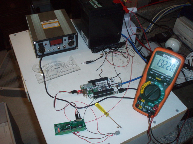
Photo 4. Acquiring Data with a Beaglebone
Page 56
Eliminated references to "both decimal and hexadecimal" -- most "counts" commands now just return hexadecimal. Added a section on processor control. Now using Ver. 3 of board. |
||
Removed Logic commands. Revised opto schematics, text. Misc. cleanup. Firmware release 140614 . Ver. 2 of board. |
||
Eliminated script description. Now points to App. Note 1. |
||
Released manual to web. Board Ver. 2, firmware release 140525 |
||
Local Release. Board Ver. 2, firmware release 140522 . |
||
First major revision |
||
Initial Release |
Copyright © 2014, Bob Nash.
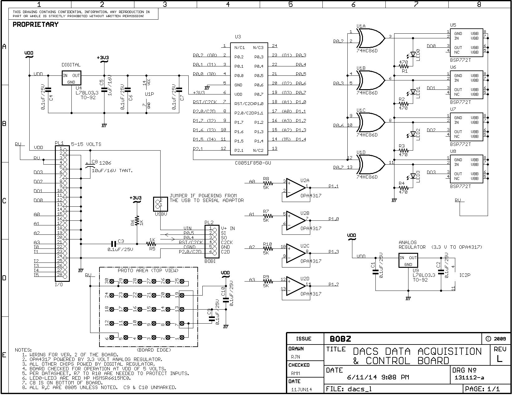